
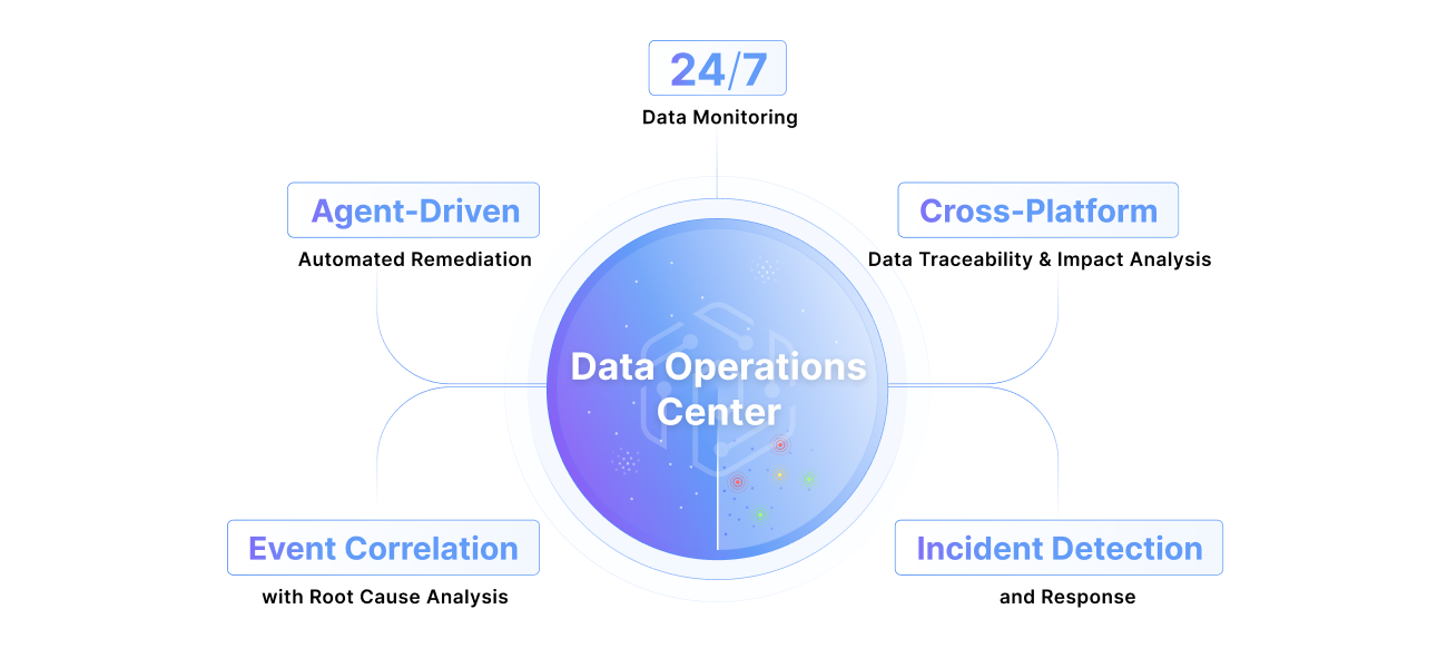
What is a data operations center?
Learn MoreWhat is a data operations center?
Learn More

Data Profiling Techniques: Best Practices
Data profiling examines a data set to derive conclusions about the data's quality, content, and completeness. These insights help improve data management, analytics, and quality. Profiling can occur at various stages of the data lifecycle, for example:
- Before data integration, evaluation of source quality and reliability is needed.
- Post-data ingestion and transformation—inspection of transformation/conversion accuracy.
Organizations implement data profiling techniques to ensure data quality and integrity and consequently improve data’s business value.
Data profiling techniques may vary significantly, depending on the objective or investigative purpose. This article explores several techniques including practical implementation examples.
Summary of key data profiling techniques
#1 Data structure analysis
Data structure analysis examines the arrangement of data and the relationship between various data objects while keeping in mind the intended business use of data. Its primary purpose is to understand how efficiently and accurately data is stored.
Data structures analysis gives companies the ability to improve on the following:
- Data integrity: Efficient data organization indicates that data follows specific constraints and rules that reduce errors and increase reliability.
- Performance: Data organization reduces performance-related bottlenecks and inefficiencies: For example, you can identify potential indexing opportunities to improve retrieval speeds by analyzing the relationships between commonly used columns.
- Data governance: Well-defined structures are easier to manage, govern, and audit.
Let’s now look at some integral structure profiling techniques and associated examples using Python and Spark. For our examples, let’s assume we are analyzing data containing information about hypothetical customers. First, let's create a Spark session and initialize a data frame.
from pyspark.sql import SparkSession
from pyspark.sql.functions import col, count, countDistinct, isnull

spark = SparkSession.builder \
	.appName("Data Structure Analysis") \
	.getOrCreate()

data = [
	(1, 'Alice', 29, 'New York'),
	(2, 'Bob', 25, 'Los Angeles'),
	(3, 'Charlie', None, 'Chicago'),
	(4, 'David', 29, 'New York'),
	(5, 'Eve', 25, 'Los Angeles'),
	(6, 'Frank', 29, 'New York'),
	(7, 'Grace', None, 'Chicago'),
	(8, 'Heidi', 30, 'New York'),
	(9, 'Ivan', 25, 'Los Angeles'),
	(10, 'Judy', 29, 'New York')
]

columns = ["id", "name", "age", "city"]
df = spark.createDataFrame(data, columns)
Column profiling
Column profiling involves the analysis of individual columns present in a dataset. It investigates data type consistency, uniqueness, missing values, etc. For our example, we look at each column to find the count, the number of distinct values, and the number of missing values.
print("Column Profiling:")
for column in df.columns:
    print(f"Column: {column}")
    df.select(
        count(col(column)).alias("count"),
        countDistinct(col(column)).alias("distinct_count"),
        count(isnull(col(column))).alias("null_count")
    ).show()
Key analysis
Key analysis is responsible for identifying primary and foreign keys in a database.
- Analysis of primary keys checks that there are no duplicates.
- Analysis of foreign keys ensures that relationships with other tables have been correctly established.
In our simple example, we only identify the primary key (id) and search for any duplicate keys.
print("Key Analysis:")
primary_key = "id"
df.groupBy(primary_key).count().filter(col("count") > 1).show()
Dependency analysis
Dependency analysis examines dependencies between columns. It gives engineers an understanding of a column's impact on another.
For example, if you had a dataset based on TV viewership, you would likely see a strong correlation between the ‘age’ and ‘TV show’ columns. For our example, we can conduct an arbitrary profiling of the relationship between age and city columns.
print("Dependency Analysis:")
grouped_df = df.groupBy("age").agg(countDistinct("city").alias("distinct_cities"))
grouped_df.show()
{{banner-large-2="/banners"}}
#2 Content profiling
Content profiling inspects a dataset's actual values to provide data engineers with insight into distribution, quality, and anomalies. The benefits of involving content profiling in your data profiling workflows include:
- Informed decision-making: Improved insights and reporting capabilities from examining content leads to more calculated decision-making by business units.
- Better data quality: A deep analysis of data values informs users about errors and anomalies before they impact downstream processes.
- Easier data integration: Profiling content allows you to standardize values and eliminate erroneous data. Integrating data into other locations becomes easier.
Let’s look at an example of content profiling on a basic data set containing information about an online student course. Once again, we use Python and Spark to initialize a dataframe.
from pyspark.sql import SparkSession
from pyspark.sql.functions import col, when, count, isnan, regexp_extract
from pyspark.sql.types import StructType, StructField, IntegerType, StringType, FloatType, BooleanType, DateType
import pyspark.sql.functions as F

spark = SparkSession.builder \
    .appName("Content Profiling Example") \
    .getOrCreate()

data = [
    (1, 'Alice', 29, 'alice@example.com', '2021-01-01', True, 85.5, 'A'),
    (2, 'Bob', 25, 'bob@example', '2021-02-15', False, 90.0, 'B'),
    (3, 'Charlie', None, None, '2021-03-10', True, 78.5, 'A'),
    (4, 'David', 30, 'david@example.com', 'not_a_date', True, None, 'B'),
    (5, 'Eve', 22, 'eve@example.com', '2021-04-22', False, 88.0, 'C')
]

schema = StructType([
    StructField("id", IntegerType(), nullable=False),
    StructField("name", StringType(), nullable=True),
    StructField("age", FloatType(), nullable=True),
    StructField("email", StringType(), nullable=True),
    StructField("signup_date", StringType(), nullable=True),
    StructField("is_active", BooleanType(), nullable=False),
    StructField("score", FloatType(), nullable=True),
    StructField("category", StringType(), nullable=True)
])

df = spark.createDataFrame(data, schema)
Data type distribution
Data type distribution helps engineers understand the variation of data types (strings, integers, etc.) among columns. Such type profiling reveals inaccuracies and misplacements in the column values.
For example, once you have a data type distribution constructed, it would be easy to flag a misplaced “string” value in a column of “floats”. For our online course example, you could develop a data type distribution to execute the following code:
print("Data Type Distribution:")
data_types = df.dtypes
for column, dtype in data_types.items():
    print(f"Column: {column}, Data Type: {dtype}")

type_counts = df.select([F.data_type(col(column)).alias(column) for column in df.columns]).groupBy(df.columns).count()
The above profiling gives us the data type associated with each column and the number of each type in the data set.
Pattern recognition
Pattern recognition looks for superficial patterns among column values (not business or statistical-related patterns). These patterns could be email, date, or customized formats for integers, floats, etc. Again, these established patterns make it easy for engineers to identify non-conforming values before they cause runtime errors or other problems. The below code shows how to profile the email and date values of the example data by pattern.
print("\nPattern Recognition:")

valid_emails = df.filter(regexp_extract(col('email'), r'^[\w\.-]+@[\w\.-]+$', 0) != "")
print("Valid Emails:")
valid_emails.select("email").show()

valid_dates = df.filter(F.to_date(col('signup_date'), 'yyyy-MM-dd').isNotNull())
print("Valid Dates:")
valid_dates.select("signup_date").show()
Outlier detection
Detecting outliers by establishing mean or standard values for columns helps identify data anomalies. These anomalies are not always erroneous, but flagging them eliminates the rare cases in which they are. Outlier detection is also very beneficial when dealing with large data volumes.
The below code creates a lower and outer bound for the student age column by calculating the interquartile range.
print("\nOutlier Detection:")

age_stats = df.select("age").describe().collect()
Q1 = float(age_stats[4][1])
Q3 = float(age_stats[6][1])
IQR = Q3 - Q1

lower_bound = Q1 - 1.5 * IQR
upper_bound = Q3 + 1.5 * IQR

outliers = df.filter((col('age') < lower_bound) | (col('age') > upper_bound))
print("Detected Outliers in Age:")
outliers.select("id", "age").show()
#3 Quality profiling
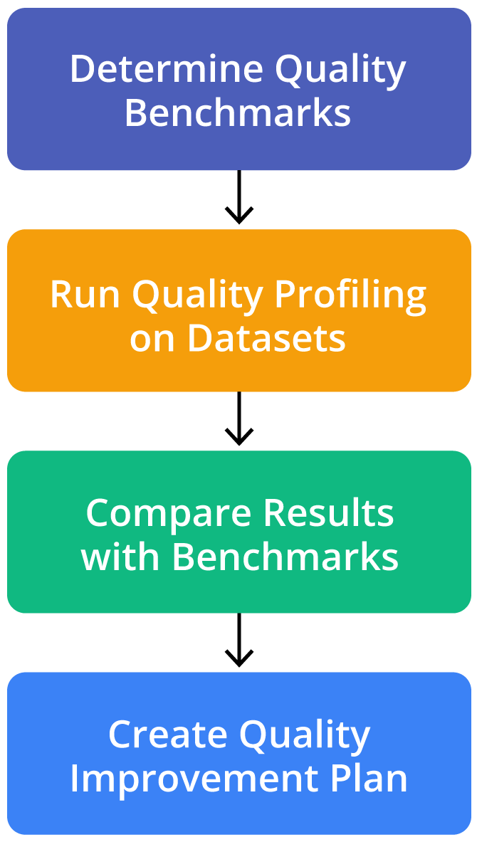
Quality profiling is the practice of setting benchmarks for data accuracy and completeness and comparing the actual values against them. These standards help organizations progressively improve data quality for improved business decisions and activities.
A typical quality profiling process starts with defining quality benchmarks in collaboration between engineers and business analysts/stakeholders to give quality requirements a more rounded perspective. Once benchmarks are established, quality profiling scripts are run on existing datasets and results are recorded and organized. Engineers look at these results along with business stakeholders, and a quality improvement plan is developed if needed. The quality profiling process should be performed periodically, especially when dealing with frequently transformed and modified data.
With more projects becoming highly data-driven, data quality is currently a sensitive and significant aspect of data engineering. Manual oversight of data quality can be cumbersome and error-prone. For this reason, using a data quality framework can help teams judge quality and quickly find anomalies. Database engineers can configure the framework to flag anomalies and sound alerts when data quality is being compromised.
The Pantomath platform allows users to integrate profiling and quality checks into their data pipelines.
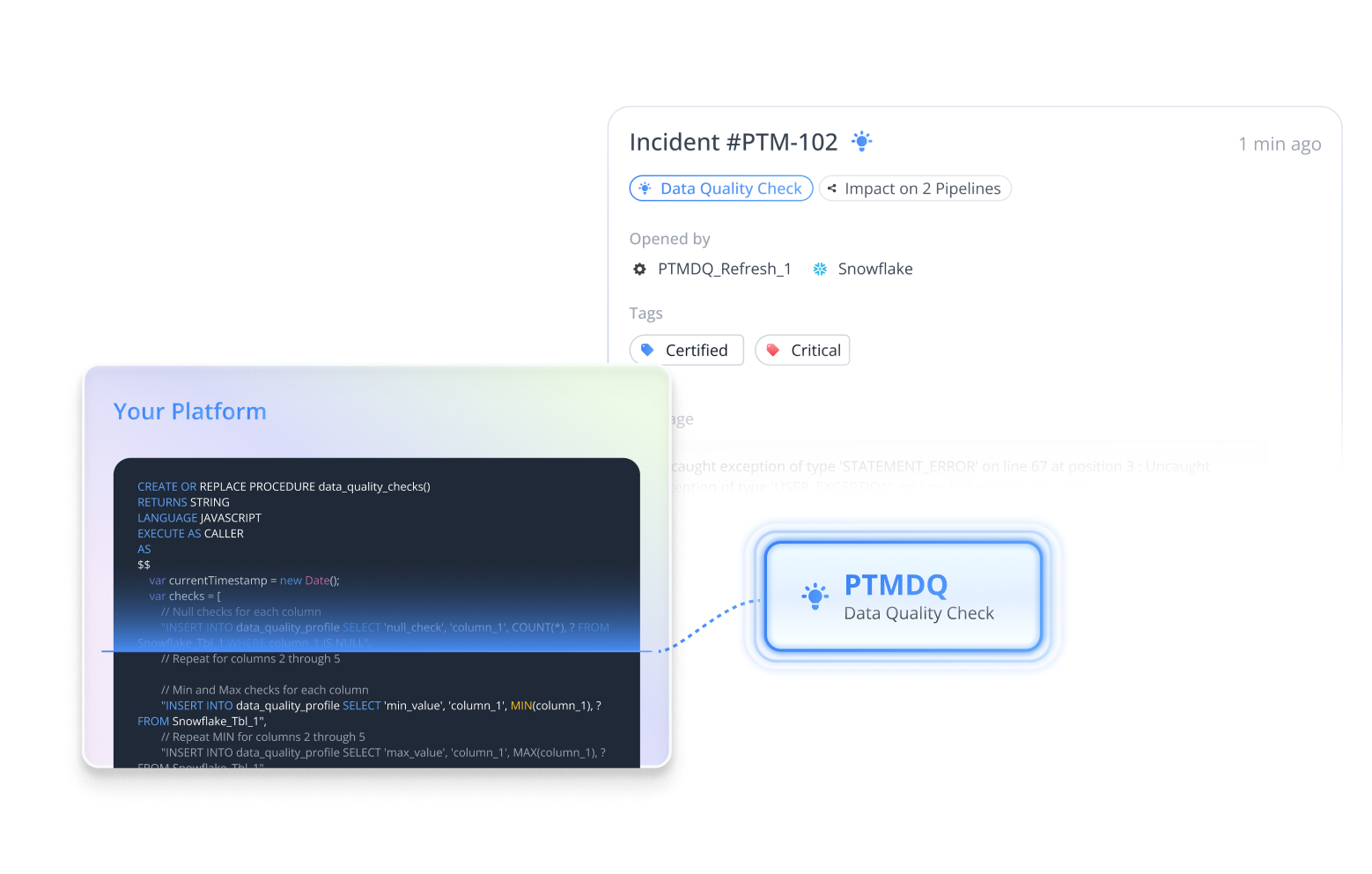
Pantomath also specializes in providing users with pipeline traceability, which quickly pinpoints the source of specific quality issues, giving users an understanding of both the root cause and the downstream impact of a data quality issue. Pantomath integrates seamlessly into many popular data technologies, such as Kafka, Databricks, Snowflake, Azure Data Factory, dbt, and Talend.
Data quality benchmarks
Developers must collaborate with business users and analysts when setting benchmarks to create realistic targets. Typical benchmarks set to gauge the quality of production data are:
Accuracy
Actual values must be within or close to the accepted range of values.
For example, looking at the database of students studying at a high school, the accepted age range is between 14 and 18. Any values outside this range should be flagged to engineers.
Completeness
The presence of all required data in a data set.
For example, in the loyalty program database of a store’s customers, the fields of “name”, “email,” and “phone number” must always be present. Entries without any of these values should be flagged when quality is profiled.
Consistency
Identical values should be consistently entered among multiple datasets.
For example, a customer’s identity details in order history should be the same as in his user profile.
#4 Statistical profiling
Statistical profiling uses statistical functions to examine the properties of a dataset further. Statistical profiling helps users understand their data in terms of distribution, patterns, and underlying trends. While this type of profiling helps identify anomalies, outliers, and erroneous data, it is most beneficial in providing reliable insights into business and market conditions. Such insights promote calculated and informed decision-making.
Let’s once again look at a sample dataset of customer purchases and carry out a few statistical profiles using Python and Spark.
from pyspark.sql import SparkSession
from pyspark.sql.functions import col, count, mean, stddev, min, max, expr
import pyspark.sql.functions as F

spark = SparkSession.builder \
    .appName("Statistical Profiling Example") \
    .getOrCreate()

data = [
    (1, 25, 100.50, 'Electronics', '2023-01-01'),
    (2, 30, 200.75, 'Clothing', '2023-01-02'),
    (3, 22, 50.00, 'Groceries', '2023-01-03'),
    (4, 35, 300.00, 'Electronics', '2023-01-04'),
    (5, 28, 150.25, 'Clothing', '2023-01-05'),
    (6, 40, 400.00, 'Electronics', '2023-01-06'),
    (7, 22, 20.00, 'Groceries', '2023-01-07'),
    (8, 30, 250.50, 'Clothing', '2023-01-08'),
    (9, 35, 120.00, 'Groceries', '2023-01-09'),
    (10, 45, 500.00, 'Electronics', '2023-01-10')
]

columns = ["customer_id", "age", "purchase_amount", "product_category", "purchase_date"]

df = spark.createDataFrame(data, columns)

df.show()
Columnar statistics
Columnar statistical evaluation provides essential summaries and numerical analyses of individual columns. Some statistics usually calculated are mean, median, min/max, and percentiles. Such results give engineers and analysts a better idea of their product demographics and hint at what changes might be required from a business perspective.
print("Columnar Statistics:")
column_stats = df.select(
    count(col("purchase_amount")).alias("Total Purchases"),
    mean(col("age")).alias("Average Age"),
    stddev(col("age")).alias("Age Std Dev"),
    min(col("purchase_amount")).alias("Min Purchase Amount"),
    max(col("purchase_amount")).alias("Max Purchase Amount")
)
The above code calculates the total purchase amount, average age, standard deviation of age, and min/max purchase amounts.
Correlation analysis
Analyzing the relationship between the values of different columns provides strategic insights. Positive correlation implies a higher degree of dependency between two columns, while negative correlation implies the opposite. No correlation can also give us meaningful information.
For example, an online toy-selling business would be interested in analyzing the correlation between certain model lines of toys and the ages of children playing with them to understand if they are marketing the product to the right buyer group.
print("Correlation Analysis:")
correlation_age_purchase = df.stat.corr("age", "purchase_amount")
print(f"Correlation between Age and Purchase Amount: {correlation_age_purchase}")
In our customer-purchases example, you can use Sparks’s stat.corr()function to calculate the correlation between age and purchase amount. The above example returns a correlation of around 0.85 implying a high degree of dependency between the two columns.
#5 Advanced profiling using ML/AI
From a broad perspective, artificial intelligence brings the following to standard data profiling:
- Enhanced data quality: The ability to fine-tune the profiling level you require and automate functions as and when data is ready.
- Predictive insights: Predicting where data anomalies might occur and how to prevent them from re-occurring.
- Scalability: When dealing with big data projects, AI optimizes real-time profiling.
Let’s look at a simple example to show how machine learning algorithms assist with anomaly detection using a sample dataset holding purchase transactions.
from pyspark.sql import SparkSession
from pyspark.sql.functions import col, when

spark = SparkSession.builder \
    .appName("Anomaly Detection Example") \
    .getOrCreate()

data = [
    (1, 100.0, "2023-01-01"),
    (2, 150.0, "2023-01-02"),
    (3, 200.0, "2023-01-03"),
    (4, 250.0, "2023-01-04"),
    (5, 300.0, "2023-01-05"),
    (6, 10000.0, "2023-01-06"),  # Anomaly
    (7, 150.0, "2023-01-07"),
    (8, 200.0, "2023-01-08"),
    (9, 175.0, "2023-01-09"),
    (10, 300.0, "2023-01-10"),
]

columns = ["transaction_id", "amount", "date"]

df = spark.createDataFrame(data, columns)

df.show()
After initializing a data frame, we train the isolation forest model.
from pyspark.ml.feature import VectorAssembler
from pyspark.ml.iforest import IsolationForest

assembler = VectorAssembler(inputCols=["amount"], outputCol="features")
df_features = assembler.transform(df)

iforest = IsolationForest(contamination=0.1)
model = iforest.fit(df_features)

predictions = model.transform(df_features)

predictions.select("transaction_id", "amount", "prediction").show()
The isolation forest algorithm finds the purchase with Id 6 to be the anomaly due to its high purchase amount. Machine learning algorithms can find anomalies in real time and in isolation instead of looking at the whole dataset with every value profile. Such a technique is helpful when analyzing live events like stock trades within an exchange system to identify fraudulent transactions.
Importance of data profiling
Having gone over various profiling techniques, the goals of profiling data always remain the same:
- Improved decision-making: Uniformly and accurately profiled data provides analysts with more information about customers, sales conversions, and other business and marketing-related factors.
- Higher data quality: Profiled data allows engineers to identify erroneous and anomalous data, improve data transformations and management and improve data quality.
- Data governance: Periodic profiling of data allows engineers and data scientists to understand their organization's datasets better and maintain strict controls on data access and modification. Such governance also keeps data management in line with industry standards.
While data profiling provides many benefits for data management, it must also be conducted with caution. Manual profiling of complex and voluminous data leads to unintentional data tampering. Data profiling and quality frameworks such as Pantomath automate profiling and ease the burden of manual profiling on engineers.
{{banner-small-5="/banners"}}
Last thoughts
Data profiling is an essential step in the data lifecycle. It helps organizations understand their data more deeply and ultimately leads to better decision-making. From the point of view of engineers and data scientists, data profiling is the first step in improving data quality, promoting efficient transformations and enhanced analytics. Manual profiling, however, can become complex and cumbersome due to the large number of necessary techniques. Data quality frameworks like Pantomath can automate these processes, making them automated and less error-prone.