Data Pipeline Automation Best Practices

The growing challenge of processing a mix of data sources, formats, and velocity in enterprises has led to the mainstream adoption of automated data pipelines designed to streamline data ingestion, integration, transformation, analysis, and reporting. 

Modern data pipeline automation goes beyond job scheduling, dependency mapping, distributed orchestration, and storage management – the staples of pipeline automation – to include data observability and pipeline traceability features that ensure data quality using anomaly detection, error detection, fault isolation, and alerting.

This article starts with a brief primer on data pipeline concepts and delves into the new functionalities of modern automated data pipelines with explanations and hands-on examples.

Summary of key data pipeline automation concepts

Why automate data pipelines?

As the number of columns, tables, and dependencies grows from dozens to hundreds, manual data processing methods become increasingly impractical, diminishing the scope of data monitoring to merely samples of the entire data set.

Automated pipelines use data checks such as schema validation and data quality checks to ensure that only accurate data is processed. For example, they can set up validation rules that automatically check data formats, ranges, and mandatory fields in semi-structured data, catching errors that might have slipped through manual checks. 

Dealing with large datasets requires the ability to correct errors automatically. Automated pipelines can trigger corrective actions without human intervention. For example, automation can detect when data flow slows and reroute the data through a backup source to ensure continuous operation. This self-healing capability is key for maintaining uninterrupted and accurate data processing. 

Types of data pipelines

This section provides a quick refresher on the basic data pipeline concepts before delving into the challenges of managing data pipelines and presenting automation techniques. 

Data pipelines differ along a few dimensions of comparison. 

1. The processing methods can be real-time (or streaming), batch and micro-batch
2. The infrastructure used for deployment might be private, public, or hybrid clouds
3. The data might be transformed before loading or storing (ETL) or after (ELT)

As we begin to review the differences, remember that a typical large enterprise environment combines these approaches to data processing.

Let’s start by quickly reviewing the processing methods used in data pipelines:

Next, let’s take a quick look at typical data processing deployment methods:

Finally, let’s compare the two typical approaches to data transformation, ETL and ELT. Remember that their use is not mutually exclusive, and data engineers often mix the two methods depending on the types of data sources. 

Pipeline data automation functionalities

This section will examine the components shown in the diagram below that automate data pipelines, starting with the three icons at the bottom from left to right.

Directed Acyclic Graph (DAG)

A Directed Acyclic Graph (DAG) is a graphical representation of a workflow in which tasks or processes are depicted with their dependencies as directed edges (thus “directed”) that can’t be cycled in a loop (thus “acyclic”). It’s a flowchart where the arrows indicate the order of task execution. 

They are required in complex environments where keeping track of dependencies in the data pipeline workflow is impractical. It also helps with job scheduling (the order for scheduling), distributed orchestration and parallel processing (covered in the next section of our article), error handling (reporting errors upstream), and pipeline monitoring (de-duplication of alerts). 

A typical data pipeline DAG might include tasks like:

1. Extract data from a CSV file
2. Transform data using SQL
3. Load the result into a data warehouse
4. Perform calculations 
5. Generate a report

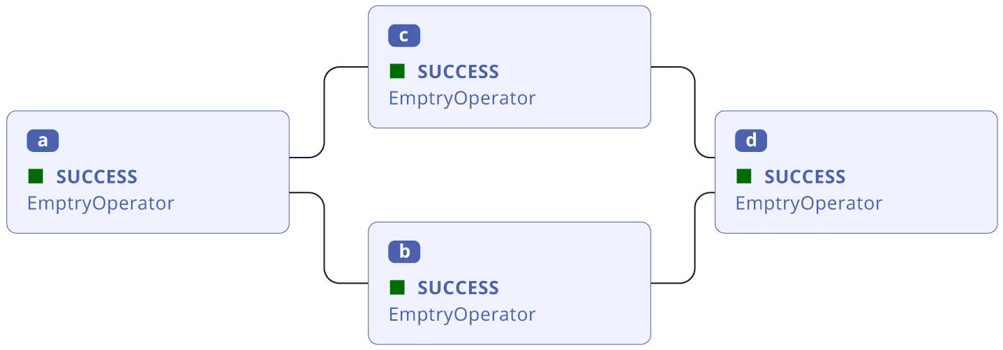
These tasks would be represented with their dependencies (e.g., the calculations must be completed before the report is generated).

Below is the most basic example of dependencies tracked by DAG where B and C depend on A and D depends on both B and C to complete, but B and C can run in parallel:

Using Apache Airflow as an example, below is a Python example of declaring dependencies in Airflow using DAG concepts. 

Below are the steps implemented in this code snippet.

• Imports the required modules from Airflow.
• Sets default parameters for the DAG, including owner, start date, email notifications, retries, etc.
• Defines the DAG with a unique ID, default arguments, description, and schedule interval.
• Creates two BashOperator tasks, t1, and t2, to execute as bash commands on a Linux shell prompt.
• Defines the dependency between t1 and t2 using the “>>” operator, defines a dependency, ensuring t1 runs before t2.

import airflow
from airflow.models import DAG
from airflow.operators.bash import BashOperator
from airflow.utils.dates import days_ago

# Default arguments for the DAG
default_args = {
    'owner': 'airflow',
    'depends_on_past': False,
    'start_date': days_ago(2),
    'email': ['airflow@example.com'],
    'email_on_failure': False,
    'email_on_retry': False,
    'retries': 1,
    'retry_delay': timedelta(minutes=5),
}

# Define the DAG
with DAG(
    'tutorial',
    default_args=default_args,
    description='A simple DAG',
    schedule_interval=timedelta(days=1),
) as dag:

    # Task 1: Print a message
    t1 = BashOperator(
        task_id='print_date',
        bash_command='date',
    )

    # Task 2: Print hello world
    t2 = BashOperator(
        task_id='print_hello',
        bash_command='echo "Hello World!"',
    )

    # Task dependency: t2 depends on t1
    t1 >> t2

With Airflow, the dependencies can be programmatically defined and updated. Behind the scenes, the program will create a giant graph of all data pipeline dependencies that can be used to orchestrate and parallelize task processing.

Job scheduling 

The job scheduler is the most basic functionality in an automated pipeline. The most rudimentary form of a job scheduler is built into the Linux operating system as a cron job. The example below shows how it can run an executable file every hour with a few commands.  

#!/bin/bash
# hourly_task.sh
echo "This script runs every hour: $(date)" >> /tmp/hourly_task.log
chmod +x hourly_task.sh
crontab -e

The command added to the crontab after running the above command:

0 * * * * /path/to/your/script/hourly_task.sh 

Considering the simplicity of a Linux cron job, imagine a sophisticated platform that can group executables, map dependencies, and let you define rules for triggering them based on events (like after the first job is completed) or scheduled every hour. This would result in hundreds of jobs harmoniously running in the intended sequence to ingest, transform, and analyze data through a data pipeline. 

We can define advanced triggers by using Apache Airflow again as an example and the concept of Directed Acyclic Graph (DAG) to group tasks as explained in the previous section. 

Below is a Linux Bash command doing just that using Airflow.

airflow dags trigger <dag_id> -r <run_id>

You can also write more complex code using Python to design business logic.

from airflow.api.client import Client 
client = Client() 
client.trigger_dag(dag_id='your_dag_id')

Distributed Orchestration

The core idea behind distributed processing is running jobs simultaneously across multiple computing nodes to save time. This processing approach is effective if the jobs don’t depend on one another’s results. For example, we might be transforming petabytes of data from one CSV format to JSON, in which case, we can shorten the process by breaking up the data into hundreds of chunks and running them simultaneously. 

Using Apache Spark as an example, a Spark job opens the SparkContext driver program and Cluster Master Node to assign tasks to worker nodes, as shown below.

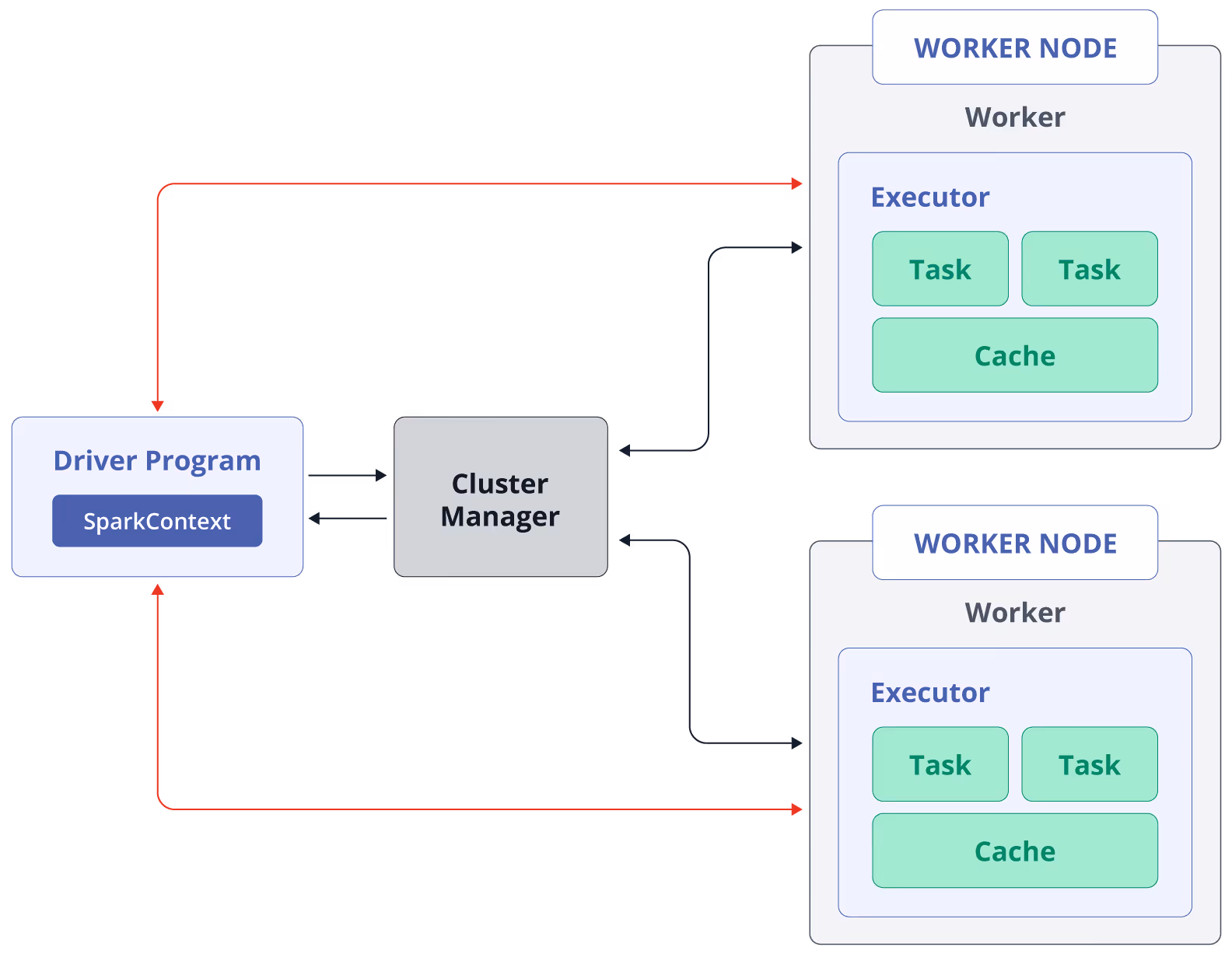
Using a word counter program for illustration, the Python code snippet below 1) partitions the text file across multiple executors, 2) creates tasks for each partition, and 3) adds up the results to calculate total work counts across the partitions.

The code's simplicity illustrates why Spark is a popular platform for orchestrating large-scale data analytics.

textFile = sc.textFile("hdfs://...") 
counts = textFile.flatMap(lambda line: line.split(" ")) \ 
           .map(lambda word: (word, 1)) \ 
           .reduceByKey(lambda a, b: a + b) 

For more context on the steps, the code reads a text file from an HDFS storage, splits it into words, counts the occurrences of each word, and produces a final Resilient Distributed Dataset (RDD) containing word-count pairs.

Data storage

The data pipeline must use different types of storage optimized for cost or performance. For example, 

• Raw data in CSV format might be stored in an AWS S3 bucket because it’s simple and inexpensive. 
• Once loaded, it might be stored in an AWS Elastic Block Store (EBS) used by the data warehouse application 
• and analyzed by the machine learning algorithm in the node’s random access memory (RAM) to shorten the computation time.
• Finally, archived data might be stored in AWS Glacier because it would cost a fraction of the cost of keeping in an AWS EBS.

However, storage management can get more dynamic in an advanced data pipeline implementation. For example, data might be 

• automatically compressed to save storage space, 
• partitioned into chunks to help with the speed of I/O access or to enable parallel processing, 
• or buffered (either in memory or on disk) to avoid being dropped between the data pipeline stages when a bottleneck slows down the processing chain, as illustrated below.

Data operations tools

The next set of data pipeline automation tools presented in the following sections is designed to enhance data accuracy and streamline data operations and are increasingly considered must-have tools in mission-critical application environments. 

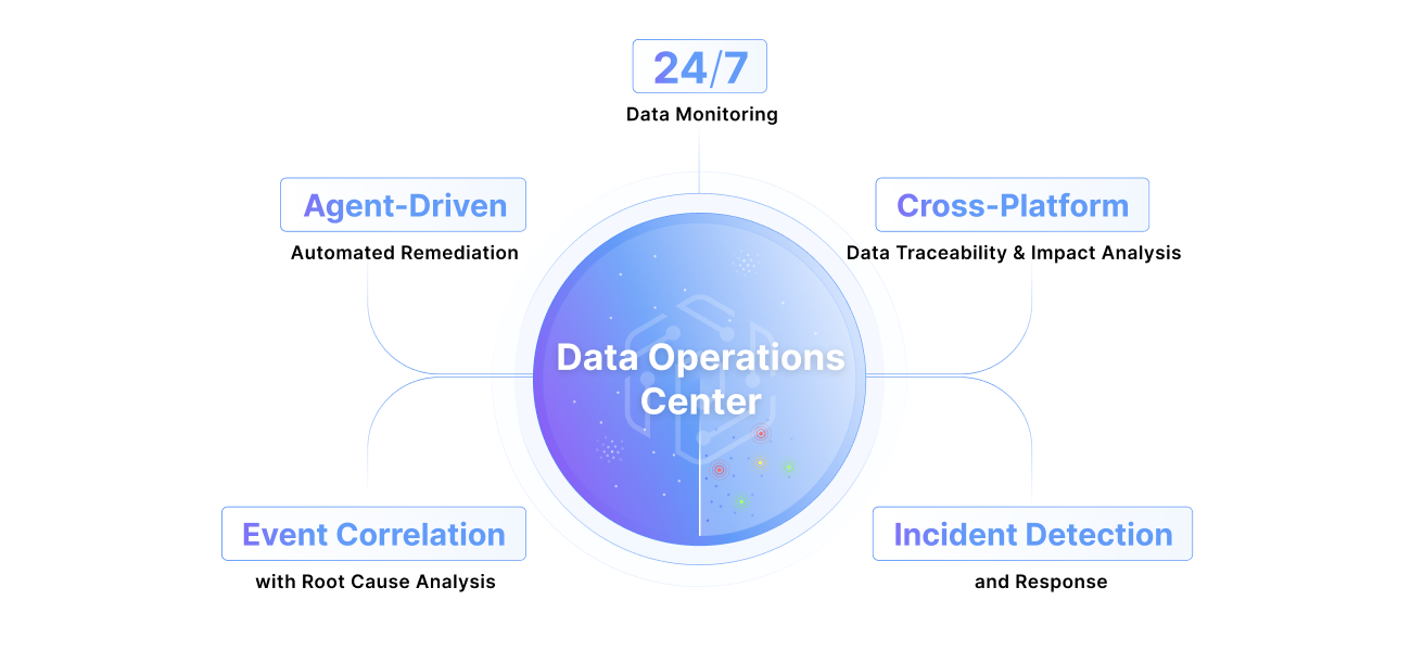
The diagram below depicts that these tools help the data operations team collaborate effectively to prevent outages, delays, and data inaccuracies.

One feature that contributes the most to the efficiency of data operations teams is automated root-cause analysis. This technique maps dependencies to correlate data quality check results (such as missing values) with operational checks (like a job failure) to isolate the upstream origin of the data quality problem. The fault isolation result is presented in an alert (or incident ticket) routed to the appropriate team for remedial action or triggers an automated script to fix recurring issues. 

DevOps teams have widely used machine learning and alerting to automate the troubleshooting process in IT infrastructure and CI/CD pipelines but such techniques have been less pervasive amongst data engineers.

Automating the troubleshooting steps shortens the mean-time-to-repair (MTTR). The following example from Pantomath’s incident management solution shows a data pipeline alert that correlates data freshness issues with “related events,” like a job failure, on which the processed data depends. 

Data quality

Data quality checks monitor the consistency, accuracy, and timeliness of data. Here are some examples organized by type:

Completeness and accuracy:

• Missing values: Identifying records with missing data in critical fields.
• Duplicate records: Detecting and removing duplicate entries.

Consistency:

• Referential integrity. Ensuring correct relationships between tables (e.g., foreign key constraints).
• Data type validation: Ensuring data conforms to expected data type (e.g., numeric, text, date).
• Column count: Detecting schema changes that might be unaccounted for.

Validity and timeliness:

• Range checks: Verifying data falls within expected ranges (e.g., a score between 0 and 10).
• Format checks: Confirming data adheres to specific formats (e.g., social security number).
• Consistency checks: Comparing data across multiple fields for consistency (e.g., city and area code).
• Uniqueness checks: Verifying unique identifiers (e.g., user ID) are unique.
• Data validation: Comparing data against predefined rules or business logic.
• Domain check. Ensuring data falls within a predefined set of values (e.g., zip code).
• Checksum verification: Validating data integrity through checksum calculations.

Data profiling

Data profiling checks are focused on data distribution and segmentation. Here are a few examples:

• Count: Number of records.
• Mean, median, mode: Core statistical attributes of numerical data.
• Standard deviation: Measure of data dispersion.
• Min, max: Range of values in a column.
• Percentiles: Distribution of data.
• Quantiles: Division of data into equal parts.

Data profiling calculations are helpful in anomaly detection to detect outlier data.

Data observability

As much as data must be verified to be consistent with the type and range of expected values, it should also be measured in terms of availability in time for transformation or analysis throughout the data pipeline, as covered by data observability checks. Here are a couple of examples:

• Data freshness: Assessing the data is up-to-date (the last modified field).
• Data volume checks: Ensuring data is complete without any missing rows or data.

Operational observability

Operational observability in data pipelines involves real-time data flow monitoring and job execution. It detects issues that can't be observed in static data, including:

• Data latency: Ensuring timely data movement between transformation points
• Data movement completeness: Verifying all records transfer as expected
• Job failure: Identifying failures and their downstream impacts in real-time
• Missed job starts: Detecting when scheduled jobs don't begin on time

Beyond issue detection, operational observability aids in troubleshooting by analyzing real-time event logs, error messages, and historical trends. It provides automated root cause analysis and recommendations to help data teams resolve issues efficiently.

Pipeline traceability

Pipeline traceability, also known as end-to-end cross-platform pipeline lineage, offers a comprehensive view of data pipelines beyond traditional data lineage. It combines application-level technical job lineage with data lineage to provide an understanding of the complete data pipeline. 

Data traceability automatically maps the interdependencies across the data pipeline to help determine the root cause. For example, data latency in the analytics stage of the pipeline might be due to a job failure a few stages back in the data transformation stage, or missing data in a field might be due to an improper schema change at the source.

By automatically mapping interdependencies across the data pipeline, pipeline traceability enables data teams to:

• Pinpoint root causes of issues anywhere in the data flow
• Resolve problems faster without manual troubleshooting
• Minimize data downtime before they propagate through the data pipeline

{{banner-large="/banners"}}

Last thoughts

Data pipeline automation has evolved in recent years. The first phase focused on establishing dependencies between tasks and running them efficiently. The next phase introduces data and operational checks to isolate the root cause of slowdowns, avoid outages, and automate remedial action.

Founded by a team of data engineers from large enterprises, Pantomath has pioneered modern techniques to boost data operations productivity. Contact an expert to learn more about how Pantomath can help.